Ed's Big Plans
URL mangling for HTML forms (a better Mediawiki search box)
Followup: This is better than my previous Mediawiki search box solution because it doesn’t require an extra PHP file (search-redirect.php) to deploy. It relies completely on URL mangling inside the HTML form on the page you are putting the search box. Previous post here.
A valid HTML form input type is “hidden”. What this means is that a variable can be set without a control displayed for it in a form. Other input types for instance are “text” for a line of text and “submit” for the proverbial submit button — both of these input types are displayed. Variables set by the “hidden” input type are treated as normal and are shipped off via the GET or POST method that you’ve chosen for the whole html form…
So, to create the following mangled URL…
https://eddiema.ca/wiki/index.php?title=Special%3ASearch&search=searchterms&go=Go
There are the following variables … with the following values:
- title … “Special%3ASearch” (%3A is the HTML entity “:”)
- search … “searchterms” (the only variable requiring user input)
- go … “Go”
The only variable that needs to be assigned from the form is “search” to which I’ve assigned the placeholder “searchterms” in the above URL.
The form thus needs only to take input for the variable “search” with a “text” type input, while “title” and “go” are already assigned– a job for the “hidden” type input.
Here’s what the simplest form for this would look like…
<form action="https://eddiema.ca/wiki/index.php" method="get">
Search Ed's Wiki Notebook:
<input name="title" type="hidden" value="Special:Search" />
<input name="search" type="text" value="" />
<input name="go" type="hidden" value="Go" />
<input type="submit" value="Search" />
</form>
Again, replace the text “Search Ed’s Wiki Notebook” with your own description and replace “https://eddiema.ca/wiki/index.php” with the form handler that you’re using– it’ll either be a bare domain, subdomain or could end with index.php if it’s a Mediawiki installation.
And that’s it! A far simpler solution than last time with the use of the “hidden” type input to assist in URL mangling.
Update: Here’s an even more improved version — this time, the end user doesn’t even see a page creation option when a full title match isn’t found. Demo (hooked up to my wiki) and Code below …
<form id="searchform" action="https://eddiema.ca/wiki/index.php" method="get">
<label class="screen-reader-text" for="s">Search Ed's Wiki Notebook:</label>
<input id="s" type="text" name="search" value="" />
<input name="fulltext" type="hidden" value="Search" />
<input id="searchsubmit" type="submit" value="Search" />
</form>
Notice that the variables “Special:Search” and “go” are not actually needed — instead, the variable “fulltext” is assigned the string “Search” — this causes mediawiki to hide the “You can create this page” option.
Add an arbitrary Mediawiki search box anywhere!
Update: A better solution that doesn’t require a separate “search-redirect.php” file has been posted here.
I’ve been looking for this solution for a long time now and I’m happy to have finally found it. Following hints from Dave Taylor and Peter De Decker, I’ve glued together a solution that doesn’t take too much effort and doesn’t require any additional hacking around in SQL.
The objective was to add a search box on the right-column navigation of this blog that would search my wiki notebook. It wasn’t until I stumbled on the above two blogs that I realized I can just mangle URLs to conduct a search on mediawikis! The specific URL used to search my wiki looks a little like this…
https://eddiema.ca/wiki/index.php?title=Special%3ASearch&search=searchterms&go=Go
It might be a bit different for your installation depending on the version that you installed and a few of your settings– to find out what it looks like, search for something and copy down the URL in the address bar.
The file “search-redirect.php” used by Wikipedia takes in your search terms, and mangles those terms into a URL conforming to the above example. It then redirects you to that constructed URL. You can find this used on the main page of Wikipedia as noted by Dave.
My search-redirect.php based on Peter’s work above is two lines long, and looks like this:
<php?
$redirect_url =
     "https://eddiema.ca/wiki/index.php?title=Special%3ASearch&search=".
     $_GET['search'].
     "&go=Go";
@header( "Location: ".$redirect_url );
?>
You probably want to place your own search-redirect.php in the root directory of your wiki installation– however, it looks to me like it doesn’t really matter since the whole URL is rewritten anyway. I bet you can put this file anywhere on the net that supports PHP. The final thing that’s missing is the search box– anything that uses this formula will work:
<form action="https://eddiema.ca/wiki/search-redirect.php" method="get">
Search Ed's Wiki:
<input type="text" name="search" />
<input type="submit" value="Search" />
</form>
Putting this code on a page with your own wiki URL as a stem instead of mine will allow you to search your own wiki from any other page.
A Chess Post – S-Chess and Omega Chess
Update: A link for Omega Chess, and a link for Seirawan Chess.
This is the first of a few posts I’d like to make about chess. In particular, this post is about two chess variants. Seirawan Chess (S-Chess) and Omega Chess. These two variants feature the familiar FIDE chess pieces along with two new pieces each. I’ll introduce each variant on their own first.
In Seirawan Chess, one starts with the familiar eight-by-eight board and opening array with the addition of two pieces set aside in reserve. These pieces are the Hawk and the Elephant. The Hawk is a Bishop and Knight compound while the Elephant is a Rook and Knight compound (a compound is a combination of pieces– a Queen is a Rook and Bishop compound). The two pieces that are set aside are placed onto the board when a player moves a piece from the back rank. The piece being dropped onto the board thus occupies the square in the back rank that has just been vacated. One can only place a single reserved piece in a given move. During a castle if the player so chooses, a reserved piece may be dropped on either the King’s or the Rook’s original square; it is not permitted to drop both reserved pieces during a castle.
In Omega Chess, one starts with a ten-by-ten board and an opening array that is flanked by the addition of a Champion and the Champion’s Pawn. The board is also extended diagonally by a single square in each of the four corners– these corner squares are occupied by a Wizard each. In the opening array, each piece is placed behind a Pawn with the exception of the Wizard. The Champion may move one step orthogonally, leap two steps orthogonally or leap two steps diagonally. The Wizard may move one step diagonally or leap (1, 3) — whereas a Knight leaps (1, 2). The Wizard is hence colour bound. The special corner Wizard squares are not actually special– they are just part of the board topology and can be used by all other pieces (except the Rook which cannot leap or slide diagonally into those spots).
For the fun of it, I have been playing Omega Chess with Seirawan Chess dropped pieces and it’s worked quite well so far. The size of the board accommodates well the Seirawan compounds. Additionally, I have been considering a house rule about dropping the Seirawan pieces– perhaps it shouldn’t be allowed that a dropped piece immediately defend the piece that dropped it. For instance, a Bishop dropping a Hawk makes for a very tough defense. A Wizard dropping a Hawk should be allowed however if the Wizard made its oblong (1, 3) leap.
If you see me walking around with a big black tube, I’m probably carrying this chess set. Challenge me to a game 😀
I’ll post some photos and such soon. The design of all the pieces from both sets is remarkably soothing and fits very well into the Staunton style. I was very lucky to discover that the Seirawan pieces are each appropriately tall compared to the Queen of the Omega Chess set I purchased.
One final thing– I decided to score the pieces in this combined game based on the mobility of each of the pieces on the ten-by-ten board. Here are my findings…
| Score | Piece | Remark |
| 29.40 | Queen | FIDE |
| 23.76 | Elephant | Seirawan |
| 18.00 | Rook | FIDE |
| 17.16 | Hawk | Seirawan |
| 11.40 | Bishop | FIDE |
| 9.36 | Champion | Omega |
| 8.28 | Wizard | Omega |
| 6.84 | King | FIDE |
| 5.76 | Knight | FIDE |
The score is proportional to the total number of squares controlled by a piece calculated for every square it can occupy in the ten-by-ten grid. Aside from giving a general impression of how one would rank a piece against other pieces, there’s not really a lot that one can tell from this scheme. In this scheme, the Seirawan pieces rank high, and the Omega pieces rank low but only due to their finite ranges. Leapers’ attacks have the distinct advantage of being immune to blocking.
That’s all for now, back to work.
The Computational Bio & Chem Group (SOLVER Revisited)
A Revisitation
In the beginnings of the Winter semester, I had an idea to start up a undergraduate/graduate student group that would provide a scaffold for faster, computer assisted research.
The semester was simply too full for me to try and get it running at that time. I’m tempted to do some work on it later this semester, after I’ve gotten more of my thesis done.
The basic idea is as follows. Faculty and graduate students in the biology and chemistry departments often have the need to analyze data with some elegant computing. Whether this be as commonplace as hacking together an excel sheet to do work or learning some existing toolbox, or something slightly more in depth such as analysis in R, Python or PERL. Unfortunately, these research problems often fall by the wayside as the time commitment to learn a new software package or programming language is not trivial without a stronger computing background. Undergraduate students who are raised in the computer science environment, particularly with a bioinformatics interest have some knowledge of the research problem semantics as well as some knowledge of how to do the above analysis by using and coding software.
The “SOLVER” group would fill the gap by performing a matchmaking and coaching service. In my vision, SOLVER creates working teams of three to four– (1) one or two graduate students or faculty with a research problem, (2) one or two undergraduate students with some knowledge in bio / chem and some talent in computing, (3) an experienced coach that can recommend best practices so that the team has a good shot of solve the problem in a reasonable amount of time. In the end, the researcher gets help and a good chance at a working solution– they might even learn some programming; educational / professional / social connections are made; and the student gets an item to add to their resume. In reality, a particular research step would be executed as week-long blocks– whether this means one block or four blocks (one month) depends on the complexity of the task.
To do…
One stretch of work that I have to do is to determine the needs of the department. I wanted to do this in the middle of Winter semester but didn’t find it a priority. For this group to work, there must be research problems. Similarly, I need to determine the capabilities of potential undergraduate students. I’m learning quickly that the key here is to start small and think big (i.e. start with one group, then two, then learn about the administrative logistics, then deploy some progress tracking mechanism, then four groups and onward).
Retuning the image
The almost idealized description above suffers from a few logistical issues. First, I will now address the issue of publication credits. Because researchers must attribute tangible work (including written code and analyses), some graduate students may be hesitant to participate in the program. I don’t know if this will actually become a barrier however as a “tangible contributor” would never be the first nor the last name on a paper (this is true in all CS, Bio and Chem). Furthermore, a paper with more than one author demonstrates the ability to collaborate in a team, and fostering the experience of another student is part of our culture (e.g. co-op students etc.). That brings me to a second major issue. One of the frames that this group could find itself in is a means to circumvent or short-circuit the co-op student appointment process– a frame that I readily reject. In fact, I should hope that this group becomes a means to introduce new putative co-op students to their future advisers which may otherwise be overlooked for their differing background. Finally, there is the problem of attrition, whereby a group dwindles in size as members drop out. The only contract-based perks or penalties I can think of is really ties to the group itself (e.g. unsatisfactory work naturally results in a time out or withdrawal from the program). It is really the only tangible leverage we can offer at the outset– unsteady leverage at best (difficult to assume a reputation when none has yet been built).
Going forward
More research has to be done in terms of polling and documenting the needs of the department. Furthermore, a deeper understanding about the kinds of students we’d attract and want to appoint is needed– this allows us to understand what time commitment is reasonable (both the lower and upper limits need definition). Finally, the group must from the outset be understood as something beneficial to all parties involved. The solutions named above must be deployed at launch time to ensure minimal friction, and maximum return. First steps were made last year by introducing this idea at the BIC-iGEM meeting– BIC students are excited with this idea, wherein an entire room of a dozen students raised their hands. Furthermore, there are no other groups on campus that attempt this activity, so that SOLVER would provide a unique non-conflicted service.
Of course– this all depends on the amount of work I get done on my own thesis in the first half of the semester.
Making friends
As an aside Isabelle Lam, a student I TA’d last semester in Biol-241 (microbio) has been planning on starting a job / volunteer / coop mine for science students. I should go and bother her and see how far she’s gotten. Her project is called “SPORE”. Last I checked, her team was registering a subdomain with the university.
EDIT: I previously confused Isabelle with Lisa– this has been corrected.
Brief Hints: C# Nullable Types and Arrays, Special Double Values
Brief Hints: I wanted to show you three things in C# that I’ve been using a lot lately.
Nullable Types are a convenient language construction in C# that allows one to assign a primitive type with null…
double? someval = null;
// declares a nullable double called 'someval'.
The question mark suffixing the keyword double makes the variable someval nullable. This was originally designed so that one can retrieve values from LINQ to SQL without checking for nulls (SQL inherently makes this distinction). This could be thought of as yet another construct to make autoboxing primitives more intuitive and more entrenched in the language.
I use nullable types when I need a special ‘unassigned’ value for “find the greatest” or “find the least” kinds of loops.
When we apply Nullable Types to Arrays, we get an array of nullable primitives (arrays are already nullable, being first class objects).
double?[] somevals = new double?[10];
// declares an array called 'somevals' of ten nullable doubles.
An array of primitives is initialized with all values 0.0; whereas an array of primitve?s is initialized with nulls.
Special Double Values are also something that I’ve started using a lot. There are many algorithms I’ve been coming across that use “magic numbers” corresponding to arbitrarily high and arbitrarily low numbers. Instead of using evil magical quantities, I’ve been using Double.PositiveInfinity and Double.NegativeInfinity. C# makes it easy to assign three more special quantities: Double.NaN, Double.MinValue and Double.MaxValue.
Edit: I forgot to mention why I kept italicizing the word primitive. C# doesn’t really have primitives that are exposed to the developer– everything actually IS an object, and the illusion of boxing or not isn’t really relevant. This just makes nullable types all the more logical.
An Old Physiology Project — Operation Spinny Chair :D
I discovered this ancient report in my repository about three months ago– I’ve finally decided to put it up because it made my day reading the abstract again. This is definitely one of my prouder albeit sillier projects from the days of my undergrad.
Independent Research Project Acute centripetal acceleration is correlated with increased heart rate and R-wave amplitude
Matthew Boyle, Bryan Chung, Eddie Ma
Abstract
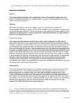
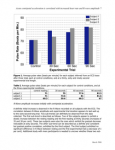
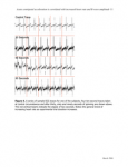
In the present study, we set out to discover the correlation between the exposure of acute centripetal acceleration in human subjects and cardiovascular function across the following three dimensions: Heart rate, R-wave amplitude and QRS interval. This was accomplished by measuring the above properties via Lead II Bipolar ECG trace, after having spun the subject at 0.8 revolutions per second in an office chair for successively, 30, 60 and 90 seconds. It was determined that heart rate showed strong positive correlation (n = 3, average increase between trials of increasing duration, 3.2 beats per minute, s = 1.8). R-wave amplitude showed positive correlation in all subjects up until and including the 60 second trial. There was no systemic correlation between duration of spin and the length of the QRS interval in any of the subjects. The heart is therefore an important effector in response to centripetal acceleration in the human model.
Key Words: electrocardiogram, QRS interval, centripetal force, R-wave amplitude, spinning office chair.
[ Download this | PDF ].Thumbnails of pages 5, 7 and 11.