On random initial weights (neural networks)
I found an old project in my archives the other day. The long and the short of it is — on occasion — if we use a three-layer back-propagation artificial neural network, initializing the hidden weight layers to larger values works better than initializing them to small values. The general wisdom is that one initializes weight layers to small values just so the bias of the system is broken, and weight values can move along, away and apart to different destination values. The general wisdom is backed by the thought that larger values can cause nets to become trapped in incorrect solutions sooner — but on this occasion, it manages to allow nets to converge more frequently.

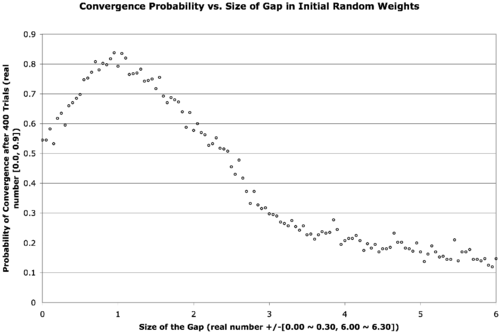
The text is a bit small, but the below explains what’s going on.
There are two neural network weight layers (2D real-valued matrices) — the first going from input-to-hidden-layer and the second going from hidden-to-output-layer. We would normally initialize these with small random values, say in the range [-0.3, 0.3]. What we’re doing here is introducing a gap in the middle of that range that expands out and forces the weights to be a bit larger. The x-axis describes the size of this gap, increasing from zero to six. The data point in the far left of the graph corresponds to a usual initialization, when the gap is zero. The gap is increased in increments of 0.05 in both the positive and negative directions for each point on the graph as we move from left to right. The next point hence corresponds to an initialization of weights in the range [-0.35, -0.05] ∨ [0.05, 0.35]. In the far right of the graph, the weights are finally randomized in the range [-6.30, -6.00] ∨ [6.00, 6.30]. The y-axis is the probability of convergence given a particular gap size. Four-hundred trials are conducted for each gap size.
The result is that the best probability of convergence was achieved when the gap size is 1.0, corresponding to weights in the random range [-1.3 -1.0] ∨ [1.0, 1.3].
What were the particular circumstances that made this work? I think this is largely dependent on the function to fit.
The Boolean function I chose was a bit of an oddball — take a look at its truth table …
| Input 1 | Input 2 | Input 3 | Output |
| 0 | 0 | 0 | 0 |
| 0 | 0 | 1 | 0 |
| 0 | 1 | 0 | 1 |
| 0 | 1 | 1 | 1 |
| 1 | 0 | 0 | 1 |
| 1 | 0 | 1 | 1 |
| 1 | 1 | 0 | 0 |
| 1 | 1 | 1 | 1 |
This comes from the function { λ : Bit_1, Bit_2, Bit_3 → (Bit_1 ∨ Bit_2) if (Bit_3) else (Bit_1 ⊕ Bit_2) }.
This function is unbalanced in the sense that it answers true more often than it answers false given the possible combinations of its inputs. This shouldn’t be too big of a problem though — we really only need any linearly inseparable function.
This project was originally done for coursework during my master’s degree. The best size for your initial weights is highly function dependent — I later found that this is less helpful (or even harmful) to problems with a continuous domain or range. It seems to work well for binary and Boolean functions and also for architectures that require recursion (I often used a gap of at least 0.6 during my master’s thesis work with the Neural Grammar Network).
Remaining parameters: training constant = 0.4; momentum = 0.4; hidden nodes = 2; convergence RMSE = 0.05 (in retrospect, using a raw count up to complete concordance would have been nicer); maximum allowed epochs = 1E5; transfer function = logistic curve.
 Ed's Big Plans