Archive for the ‘Machine Learning’ Category
My talk at Complex Adaptive Systems, Chicago (2011)
I’ve just returned from the Complex Adaptive Systems conference on Wednesday after an eight hour drive — well, most of the driving was done by Dr. Obimbo and Haochen. I presented my paper An evolutionary computation attack on one-round TEA. This paper is built on top of my course project in Computer Security (University of Guelph, Winter 2011). This is my first cryptanalysis paper, and is an aside to the bioinformatics focus of my thesis.
My slides introduce Tiny Encryption Algorithm (TEA) pretty well, along with Genetic Algorithm (GA) and Harmony Search (HS). The slides detailing the results aren’t quite as self-explanatory, but are bearable since the theme is fairly easy to establish: simpler keys are easier to break than more complicated ones.
>>> Download: CAS2011Chicago.pdf — my presentation from Chicago. <<<
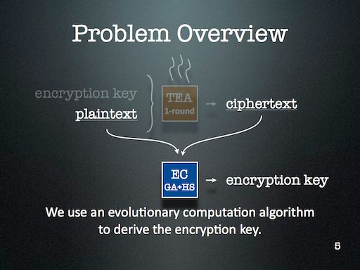
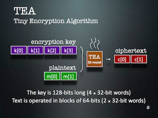
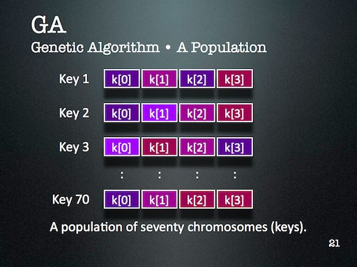
I might look at cryptanalysis again in future — but I’ll certainly use Evolutionary Computation (EC) again. It’s just too readily available in my toolkit, and is far too easy to deploy. One of the major lessons of this project that became very clear through during discussion with the audience is that the operators that are part of an EC algorithm should reflect the kind of problem we’re trying to solve. This might seem obvious at first, but I think it’s more subtle than that. For this project, HS enabled the EC to probe a keyspace with many repetitions — something that GA operators alone didn’t provide us.
In general however, the solution space is lumpy enough that using ECs against stronger encryption schemes is just not viable — unless the EC had some magic to overcome the linearly inseparable lumps. I haven’t yet met such an operator and am not convinced one way or another about its existence. I’ll certainly introduce you if I ever do bump into it 😛
Blog Author Clustering with SOMs
For the final project in Neural Networks (CIS 6050 W11), I decided to cluster blog posts based on the difference between an author’s word choice and the word choice of the entire group of authors.
>>> Attached Course Paper: Kohonen Self-Organizing Maps in Clustering of Blog Authors (pdf) <<<
A self-organizing map (Kohonen SOM) strategy was used. The words chosen to compose a given blog post defined wherein the map it should be placed. The purpose of this project was to figure out what predictive power could be harnessed given the combination of the SOM and each author’s lexicon; i.e. whether or not it is possible to automatically categorize an author’s latest post without the use of any tools besides the above.
Data: Thirteen authors contributing a total of fourteen blogs participated in the study (all data was retrieved on 2011 March 8th). The below table summarizes the origin of the data.
| Author | Posts | Lexicon | Blog Name | Subject Matter |
| Andre Masella | 198 | 7953 | MasellaSphere | Synth Bio, Cooking, Engineering |
| Andrew Berry | 46 | 2630 | Andrew Berry Development | Drupal, Web Dev, Gadgets |
| Arianne Villa | 41 | 1217 | …mrfmr. | Internet Culture, Life |
| Cara Ma | 12 | 854 | Cara’s Awesome Blog | Life, Pets, Health |
| Daniela Mihalciuc | 211 | 4454 | Citisen of the World† | Travel, Life, Photographs |
| Eddie Ma | 161 | 5960 | Ed’s Big Plans | Computing, Academic, Science |
| Jason Ernst | 61 | 3445 | Jason’s Computer Science Blog | Computing, Academic |
| John Heil | 4 | 712 | Dos Margaritas Por Favor | Science, Music, Photography |
| Lauren Stein | 91 | 4784 | The Most Interesting Person | Improv, Happiness, Events |
| Lauren Stein (Cooking) | 7 | 593 | The Laurentina Cookbook | Cooking, Humour |
| Liv Monck-Whipp | 30 | 398 | omniology | Academic, Biology, Science |
| Matthew Gingerich | 98 | 395 | The Majugi Blog | Academic, Synth Bio, Engineering |
| Richard Schwarting | 238 | 7538 | Kosmokaryote | Academic, Computing, Linux |
| Tony Thompson | 51 | 2346 | Tony Thompson, Geek for Hire | Circuitry, Electronic Craft, Academic |
†Daniela remarks that the spelling of Citisen is intentional.
In order to place the blog posts into a SOM, each post was converted to a bitvector. Each bit is assigned to a specific word, so that the positions of each bit consistently represents the same word from post to post. An on-bit represented the presence of a word while an off-bit represented the absence of a word. Frequently used words like “the” were omitted from the word bit-vector, and seldom used words were also omitted.
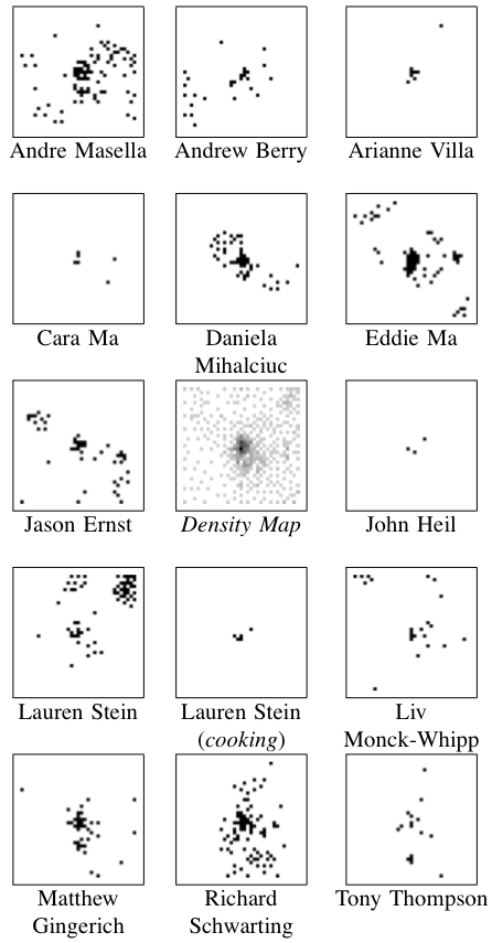 Results: The center image (in the collection to the left) is a density map where darker pixels indicates a larger number of posts — this centre map represents all of the posts made by all of the authors pooled together.
Because of the number of posts and the number of authors, I’ve exploded the single SOM image into the remaining fourteen images.
It was found that posts were most often clustered together if they were both by the same author and on the same topic. Clusters containing more than one author generally did not show much agreement about the topic.
Regions of this SOM were dominated by particular authors and topics as below.
| Region | Authors | Topics |
| Top Left | Liv | Academic Journals |
| Eddie | Software Projects | |
| Jason | Academic | |
| Top Border | Lauren | Human Idiosyncrasies |
| Richard | Linux | |
| Top Right | Lauren | Improv |
| Up & Left of Centre | Daniela | Travel |
| Centre | all | short and misfit posts |
| Right Border | Andre | Cooking |
| Just Below Centre | Matthew | Software Projects |
| Bottom Left | Andre | Language Theory |
| Andrew | Software Projects | |
| Jason | Software Projects | |
| Bottom Border | Richard | Academic |
| Bottom Right | Eddie | Web Development |
| Jason | Software Tutorials |
Discussion: There are some numerical results to go along with this, but they aren’t terribly exciting — the long and the short of it is that this project should to be repeated. The present work points towards the following two needed improvements.
First, the way the bitvectors were cropped at the beginning and at the end were based on a usage heuristic that doesn’t really conform to information theory. I’d likely take a look at the positional density of all bits to select meaningful words to cluster.
Second, all posts were included — this results in the dense spot in the middle of the central map. Whether these posts are short or just misfit, many of them can probably be removed by analyzing their bit density too.
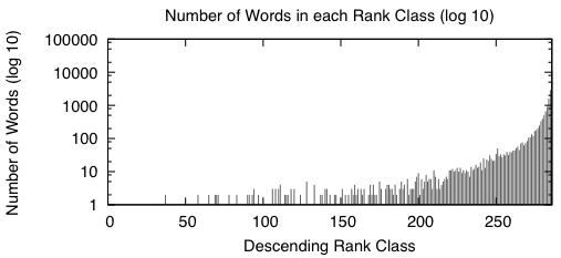
Appendix: Here are two figures that describe the distribution of the data in the word bitvectors.
 |
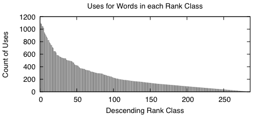 |
When we sort the words based from a high number of occurrences down to a low number of occurrences, we get graphs that look like the above two. A rank class contains all words that have the same number of occurrences across the entire study. The impulse graph on the left shows the trend for the number of unique words in each rank class. The number of words drastically increases as the classes contain fewer words. The impulse graph on the right shows the trend for the count of uses for words in a given rank class. The number of uses decreases as words become more rare.
These graphs were made before the main body of the work to sketch out how I wanted the bitvectors to behave — they verify that there was nothing unusual about the way the words were distributed amongst the data.
On random initial weights (neural networks)
I found an old project in my archives the other day. The long and the short of it is — on occasion — if we use a three-layer back-propagation artificial neural network, initializing the hidden weight layers to larger values works better than initializing them to small values. The general wisdom is that one initializes weight layers to small values just so the bias of the system is broken, and weight values can move along, away and apart to different destination values. The general wisdom is backed by the thought that larger values can cause nets to become trapped in incorrect solutions sooner — but on this occasion, it manages to allow nets to converge more frequently.
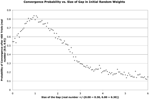
The text is a bit small, but the below explains what’s going on.
There are two neural network weight layers (2D real-valued matrices) — the first going from input-to-hidden-layer and the second going from hidden-to-output-layer. We would normally initialize these with small random values, say in the range [-0.3, 0.3]. What we’re doing here is introducing a gap in the middle of that range that expands out and forces the weights to be a bit larger. The x-axis describes the size of this gap, increasing from zero to six. The data point in the far left of the graph corresponds to a usual initialization, when the gap is zero. The gap is increased in increments of 0.05 in both the positive and negative directions for each point on the graph as we move from left to right. The next point hence corresponds to an initialization of weights in the range [-0.35, -0.05] ∨ [0.05, 0.35]. In the far right of the graph, the weights are finally randomized in the range [-6.30, -6.00] ∨ [6.00, 6.30]. The y-axis is the probability of convergence given a particular gap size. Four-hundred trials are conducted for each gap size.
The result is that the best probability of convergence was achieved when the gap size is 1.0, corresponding to weights in the random range [-1.3 -1.0] ∨ [1.0, 1.3].
What were the particular circumstances that made this work? I think this is largely dependent on the function to fit.
The Boolean function I chose was a bit of an oddball — take a look at its truth table …
| Input 1 | Input 2 | Input 3 | Output |
| 0 | 0 | 0 | 0 |
| 0 | 0 | 1 | 0 |
| 0 | 1 | 0 | 1 |
| 0 | 1 | 1 | 1 |
| 1 | 0 | 0 | 1 |
| 1 | 0 | 1 | 1 |
| 1 | 1 | 0 | 0 |
| 1 | 1 | 1 | 1 |
This comes from the function { λ : Bit_1, Bit_2, Bit_3 → (Bit_1 ∨ Bit_2) if (Bit_3) else (Bit_1 ⊕ Bit_2) }.
This function is unbalanced in the sense that it answers true more often than it answers false given the possible combinations of its inputs. This shouldn’t be too big of a problem though — we really only need any linearly inseparable function.
This project was originally done for coursework during my master’s degree. The best size for your initial weights is highly function dependent — I later found that this is less helpful (or even harmful) to problems with a continuous domain or range. It seems to work well for binary and Boolean functions and also for architectures that require recursion (I often used a gap of at least 0.6 during my master’s thesis work with the Neural Grammar Network).
Remaining parameters: training constant = 0.4; momentum = 0.4; hidden nodes = 2; convergence RMSE = 0.05 (in retrospect, using a raw count up to complete concordance would have been nicer); maximum allowed epochs = 1E5; transfer function = logistic curve.
SOM Indexing Logic
Update: Added some code too.
Brief: A classmate and I started talking about how we implemented the Kohonen Self Organizing Maps (SOM)s. I used C and indexed first the rows and the columns of the SOM before the index corresponding to the weight vectors (same as the index for the input vectors); he used C++ and indexed the weight vectors first before the columns and the rows.
Either way, we could use a three-deep array like this (switching the indexers as appropriate) …
const double low = 0.0; // minimum allowed random value to initialize weights
const double high = 1.0; // maximum allowed random value to initialize weights
const int nrows = 4; // number of rows in the map
const int ncolumns = 4; // number of columns in the map
const int ninputs = 3; // number of elements in an input vector, each weight vector

double*** weight; // the weight array

weight = calloc(nrows, sizeof(double**));
for(int r = 0; r < nrows; r ++) {
    weight[r] = calloc(ncolumns, sizeof(double*));
    for(int c = 0; c < ncolumns; c ++) {
        weight[r] = calloc(ninputs, sizeof(double));
        for(int i = 0; i < ninputs; i ++) {
            weight[r][i] =
            (((double)random() / (double)INT_MAX) * (high - low)) + low;
        }
    }
}
In the below diagram, the left side is a schematic of his approach and the right side is a schematic of my approach.
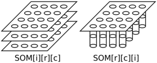
Figure above: SOM Indexing — Left (his): SOM indexed as input, row, column; Right (mine): SOM indexed as row, column, input.
Both schematics in the above diagram have four rows and four columns in the map where each weight (and input) vector has three elements.
I think my logic is better since we’ll often be using some distance function to evaluate how similar a weight vector is to a given input — to me, it’s natural to thus index these at the inner most nesting while looping over the rows and columns of the map.
The opposing approach was apparently used because my classmate had previously developed a matrix manipulation library. I’m actually kind of curious to take a look at it later.
SOM in Regression Data (animation)
The below animation is what happens when you train a Kohonen Self-Organizing Map (SOM) using data meant for regression instead of clustering or classification. A total of 417300 training cycles are performed — a single training cycle is the presentation of one exemplar to the SOM. The SOM has dimensions 65×65. Exemplars are chosen at random and 242 snapshots are taken in total (once every 1738 training cycles).
 Ed's Big Plans