Ed's Big Plans
Archive for the ‘Featured’ Category
On random initial weights (neural networks)
I found an old project in my archives the other day. The long and the short of it is — on occasion — if we use a three-layer back-propagation artificial neural network, initializing the hidden weight layers to larger values works better than initializing them to small values. The general wisdom is that one initializes weight layers to small values just so the bias of the system is broken, and weight values can move along, away and apart to different destination values. The general wisdom is backed by the thought that larger values can cause nets to become trapped in incorrect solutions sooner — but on this occasion, it manages to allow nets to converge more frequently.

The text is a bit small, but the below explains what’s going on.
There are two neural network weight layers (2D real-valued matrices) — the first going from input-to-hidden-layer and the second going from hidden-to-output-layer. We would normally initialize these with small random values, say in the range [-0.3, 0.3]. What we’re doing here is introducing a gap in the middle of that range that expands out and forces the weights to be a bit larger. The x-axis describes the size of this gap, increasing from zero to six. The data point in the far left of the graph corresponds to a usual initialization, when the gap is zero. The gap is increased in increments of 0.05 in both the positive and negative directions for each point on the graph as we move from left to right. The next point hence corresponds to an initialization of weights in the range [-0.35, -0.05] ∨ [0.05, 0.35]. In the far right of the graph, the weights are finally randomized in the range [-6.30, -6.00] ∨ [6.00, 6.30]. The y-axis is the probability of convergence given a particular gap size. Four-hundred trials are conducted for each gap size.
The result is that the best probability of convergence was achieved when the gap size is 1.0, corresponding to weights in the random range [-1.3 -1.0] ∨ [1.0, 1.3].
What were the particular circumstances that made this work? I think this is largely dependent on the function to fit.
The Boolean function I chose was a bit of an oddball — take a look at its truth table …
| Input 1 | Input 2 | Input 3 | Output |
| 0 | 0 | 0 | 0 |
| 0 | 0 | 1 | 0 |
| 0 | 1 | 0 | 1 |
| 0 | 1 | 1 | 1 |
| 1 | 0 | 0 | 1 |
| 1 | 0 | 1 | 1 |
| 1 | 1 | 0 | 0 |
| 1 | 1 | 1 | 1 |
This comes from the function { λ : Bit_1, Bit_2, Bit_3 → (Bit_1 ∨ Bit_2) if (Bit_3) else (Bit_1 ⊕ Bit_2) }.
This function is unbalanced in the sense that it answers true more often than it answers false given the possible combinations of its inputs. This shouldn’t be too big of a problem though — we really only need any linearly inseparable function.
This project was originally done for coursework during my master’s degree. The best size for your initial weights is highly function dependent — I later found that this is less helpful (or even harmful) to problems with a continuous domain or range. It seems to work well for binary and Boolean functions and also for architectures that require recursion (I often used a gap of at least 0.6 during my master’s thesis work with the Neural Grammar Network).
Remaining parameters: training constant = 0.4; momentum = 0.4; hidden nodes = 2; convergence RMSE = 0.05 (in retrospect, using a raw count up to complete concordance would have been nicer); maximum allowed epochs = 1E5; transfer function = logistic curve.
SOM in Regression Data (animation)
The below animation is what happens when you train a Kohonen Self-Organizing Map (SOM) using data meant for regression instead of clustering or classification. A total of 417300 training cycles are performed — a single training cycle is the presentation of one exemplar to the SOM. The SOM has dimensions 65×65. Exemplars are chosen at random and 242 snapshots are taken in total (once every 1738 training cycles).
C & Bioinformatics: ASCII Nucleotide Comparison Circuit
Here’s a function I developed for Andre about a week ago. The C function takes two arguments. Both arguments are C characters. The first argument corresponds to a degenerate nucleotide as in the below table. The second argument corresponds to a non-degenerate nucleotide {‘A’, ‘C’, ‘G’, ‘T’} or any nucleotide ‘N’. The function returns zero if the logical intersection between the two arguments is zero. The function returns a one-hot binary encoding for the logical intersection if it exists so that {‘A’ = 1, ‘C’ = 2, ‘G’ = 4, ‘T’ = 8} and {‘N’ = 15}. All of this is done treating the lower 5-bits of the ASCII encoding for each character as wires of a circuit.
| Character | ASCII (Low 5-Bits) |
Represents | One Hot | Equals |
| A |
00001 |
A | 0001 |
1 |
| B | 00010 | CGT | 1110 |
14 |
| C | 00011 | C | 0010 |
2 |
| D | 00100 | AGT | 1101 |
13 |
| G | 00111 | G | 0100 |
4 |
| H | 01000 | ACT | 1011 |
11 |
| K |
01011 | GT | 1100 |
12 |
| M | 01101 | AC | 0011 |
3 |
| N | 01110 | ACGT | 1111 |
15 |
| R | 10010 | AG | 0101 | 5 |
| S | 10011 | GC | 0110 |
6 |
| T | 10100 | T |
1000 |
8 |
| V | 10110 | ACG |
0111 |
7 |
| W | 10111 | AT |
1001 |
9 |
| Y | 11001 | CT |
1010 |
10 |
The premise is that removing all of the logical branching and using only binary operators would make things a bit faster — I’m actually not sure if the following solution is faster because there are twelve variables local to the function scope — we can be assured that at least half of these variables will be stored outside of cache and will have to live in memory. We’d get a moderate speed boost if at all.
/*
    f():
        Bitwise comparison circuit that treats nucleotide and degenerate
        nucleotide ascii characters as mathematical sets.
        The operation performed is set i intersect j.
    arg char i:
        Primer -- accepts ascii |ABCDG HKMNR STVWY| = 15.
    arg char j:
        Sequence -- accepts ascii |ACGTN| = 5.
    return char (k = 0):
        false -- i intersect j is empty.
    return char (k > 0):
        1 -- the intersection is 'A'
        2 -- the intersection is 'C'
        4 -- the intersection is 'G'
        8 -- the intersection is 'T'
       15 -- the intersection is 'N'
    return char (undefined value):
        ? -- if any other characters are placed in i or j.
*/
char f(char i, char j) {

    // break apart Primer into bits ...
    char p = (i >> 4) &1;
    char q = (i >> 3) &1;
    char r = (i >> 2) &1;
    char s = (i >> 1) &1;
    char t =  i       &1;

    // break apart Sequence into bits ...
    char a = (j >> 4) &1;
    char b = (j >> 3) &1;
    char c = (j >> 2) &1;
    char d = (j >> 1) &1;
    char e =  j       &1;

    return

    ( // == PRIMER CIRCUIT ==
        ( // -- A --
            ((p|q|r|s  )^1) &         t |
            ((p|q|  s|t)^1) &     r     |
            ((p|  r|s|t)^1) &   q       |
            ((p|    s  )^1) &   q&r&  t |
            ((p|      t)^1) &   q&r&s   |
            ((  q|    t)^1) & p&s       |
            ((  q      )^1) & p&r&s
        )
        |
        ( // -- C --
            ((p|q|r    )^1) &       s   |
            ((p|  r|s|t)^1) &   q       |
            ((p|    s  )^1) &   q&r&  t |
            ((p|      t)^1) &   q&r&s   |
            ((  q|r    )^1) &       s&t |
            ((  q|    t)^1) & p  &r&s   |
            ((    r|s  )^1) & p&q&    t
        ) << 1
        |
        ( // -- G --
            ((  q|r|  t)^1) &       s   |
            ((p|q|  s|t)^1) &     r     |
            ((p|q      )^1) &     r&s&t |
            ((p|  r    )^1) &   q&  s&t |
            ((p|      t)^1) &   q&r&s   |
            ((  q|r    )^1) & p&    s   |
            ((  q|    t)^1) & p&    s
        ) << 2
        |
        ( // -- T --
            ((p|q|r|  t)^1) &       s   |
            ((  q|  s|t)^1) &     r     |
            ((p|  r|s|t)^1) &   q       |
            ((p|  r    )^1) &   q&  s&t |
            ((p|      t)^1) &   q&r&s   |
            ((  q      )^1) & p&  r&s&t |
            ((    r|s  )^1) & p&q&    t
        ) << 3
    )
    &
    ( // == SEQUENCE CIRCUIT ==
        ( // -- A --
            ((a|b|c|d  )^1) &         e |
            ((a|      e)^1) &   b&c&d
        )
        |
        ( // -- C --
            ((a|b|c    )^1) &       d&e |
            ((a|      e)^1) &   b&c&d
        ) << 1
        |
        ( // -- G --
            ((a|b      )^1) &     c&d&e |
            ((a|      e)^1) &   b&c&d
        ) << 2
        |
        ( // -- T --
            ((a|      e)^1) &   b&c&d   |
            ((  b|  d|e)^1) & a&  c
        ) << 3
    );
}
Andre’s eventual solution was to use a look-up table which very likely proves faster in practice. At the very least, this was a nice refresher and practical example for circuit logic using four sets of minterms (one for each one-hot output wire).
Should you need this logic to build a fast physical circuit or have some magical architecture with a dozen registers (accessible to the compiler), be my guest 😀
C & Math: Sieve of Eratosthenes with Wheel Factorization
In the first assignment of Computer Security, we were to implement The Sieve of Eratosthenes. The instructor gives a student the failing grade of 6/13 for a naive implementation, and as we increase the efficiency of the sieve, we get more marks. There are the three standard optimizations: (1) for the current prime being considered, start the indexer at the square of the current prime; (2) consider only even numbers; (3) end crossing out numbers at the square root of the last value of the sieve.
Since the assignment has been handed in, I’ve decided to post my solution here as I haven’t seen C code on the web which implements wheel factorization.
We can think of wheel factorization as an extension to skipping all even numbers. Since we know that all even numbers are multiples of two, we can just skip them all and save half the work. By the same token, if we know a pattern of repeating multiples corresponding to the first few primes, then we can skip all of those guaranteed multiples and save some work.
The wheel I implement skips all multiples of 2, 3 and 5. In Melissa O’Neill’s The Genuine Sieve of Erastothenes, an implementation of the sieve with a priority queue optimization is shown in Haskell while wheel factorization with the primes 2, 3, 5 and 7 is discussed. The implementation of that wheel (and other wheels) is left as an exercise for her readers 😛
But first, let’s take a look at the savings of implementing this wheel. Consider the block of numbers in modulo thirty below corresponding to the wheel for primes 2, 3 and 5 …
| 0 | 1 | 2 | 3 | 4 | 5 | 6 | 7 | 8 | 9 |
| 10 | 11 | 12 | 13 | 14 | 15 | 16 | 17 | 18 | 19 |
| 20 | 21 | 22 | 23 | 24 | 25 | 26 | 27 | 28 | 29 |
Only the highlighted numbers need to be checked to be crossed out during sieving since the remaining values are guaranteed to be multiples of 2, 3 or 5. This pattern repeats every thirty numbers which is why I say that it is in modulo thirty. We hence skip 22/30 of all cells by using the wheel of thirty — a savings of 73%. If we implemented the wheel O’Neill mentioned, we would skip 77% of cells using a wheel of 210 (for primes 2, 3, 5 and 7).
(Note that the highlighted numbers in the above block also correspond to the multiplicative identity one and numbers which are coprime to 30.)
Below is the final code that I used.
#include <stdlib.h>
#include <stdio.h>
#include <math.h>

const unsigned int SIEVE = 15319000;
const unsigned int PRIME = 990000;

int main(void) {
    unsigned char* sieve = calloc(SIEVE + 30, 1); // +30 gives us incr padding
    unsigned int thisprime = 7;
    unsigned int iprime = 4;

    unsigned int sieveroot = (int)sqrt(SIEVE) +1;

    // Update: don't need to zero the sieve - using calloc() not malloc()

    sieve[7] = 1;

    for(; iprime < PRIME; iprime ++) {
        // ENHANCEMENT 3: only cross off until square root of |seive|.
        if(thisprime < sieveroot) {
            // ENHANCEMENT 1: Increment by 30 -- 4/15 the work.
            // ENHANCEMENT 2: start crossing off at prime * prime.
            int i = (thisprime * thisprime);
            switch (i % 30) { // new squared prime -- get equivalence class.
                case 1:
                    if(!sieve[i] && !(i % thisprime)) {sieve[i] = 1;}
                    i += 6;
                case 7:
                    if(!sieve[i] && !(i % thisprime)) {sieve[i] = 1;}
                    i += 4;
                case 11:
                    if(!sieve[i] && !(i % thisprime)) {sieve[i] = 1;}
                    i += 2;
                case 13:
                    if(!sieve[i] && !(i % thisprime)) {sieve[i] = 1;}
                    i += 4;
                case 17:
                    if(!sieve[i] && !(i % thisprime)) {sieve[i] = 1;}
                    i += 2;
                case 19:
                    if(!sieve[i] && !(i % thisprime)) {sieve[i] = 1;}
                    i += 4;
                case 23:
                    if(!sieve[i] && !(i % thisprime)) {sieve[i] = 1;}
                    i += 6;
                case 29:
                    if(!sieve[i] && !(i % thisprime)) {sieve[i] = 1;}
                    i += 1; // 29 + 1 (mod 30) = 0 -- just in step
            }
            for(; i < SIEVE; i += 30) {
                if(!sieve[i+1] && !((i+1) % thisprime)) sieve[i+1] = 1;
                if(!sieve[i+7] && !((i+7) % thisprime)) sieve[i+7] = 1;
                if(!sieve[i+11] && !((i+11) % thisprime)) sieve[i+11] = 1;
                if(!sieve[i+13] && !((i+13) % thisprime)) sieve[i+13] = 1;
                if(!sieve[i+17] && !((i+17) % thisprime)) sieve[i+17] = 1;
                if(!sieve[i+19] && !((i+19) % thisprime)) sieve[i+19] = 1;
                if(!sieve[i+23] && !((i+23) % thisprime)) sieve[i+23] = 1;
                if(!sieve[i+29] && !((i+29) % thisprime)) sieve[i+29] = 1;
            }
        }

        {
            int i = thisprime;
            switch (i % 30) { // write down the next prime in 'thisprime'.
                case 1:
                    if(!sieve[i]) {thisprime = i; sieve[i] = 1; goto done;}
                    i += 6;
                case 7:
                    if(!sieve[i]) {thisprime = i; sieve[i] = 1; goto done;}
                    i += 4;
                case 11:
                    if(!sieve[i]) {thisprime = i; sieve[i] = 1; goto done;}
                    i += 2;
                case 13:
                    if(!sieve[i]) {thisprime = i; sieve[i] = 1; goto done;}
                    i += 4;
                case 17:
                    if(!sieve[i]) {thisprime = i; sieve[i] = 1; goto done;}
                    i += 2;
                case 19:
                    if(!sieve[i]) {thisprime = i; sieve[i] = 1; goto done;}
                    i += 4;
                case 23:
                    if(!sieve[i]) {thisprime = i; sieve[i] = 1; goto done;}
                    i += 6;
                case 29:
                    if(!sieve[i]) {thisprime = i; sieve[i] = 1; goto done;}
                    i += 1;
            }
            for(; i < SIEVE; i += 30) {
                if(!sieve[i+1]) {thisprime = i+1; sieve[i+1] = 1; goto done;}
                if(!sieve[i+7]) {thisprime = i+7; sieve[i+7] = 1; goto done;}
                if(!sieve[i+11]) {thisprime = i+11; sieve[i+11] = 1; goto done;}
                if(!sieve[i+13]) {thisprime = i+13; sieve[i+13] = 1; goto done;}
                if(!sieve[i+17]) {thisprime = i+17; sieve[i+17] = 1; goto done;}
                if(!sieve[i+19]) {thisprime = i+19; sieve[i+19] = 1; goto done;}
                if(!sieve[i+23]) {thisprime = i+23; sieve[i+23] = 1; goto done;}
                if(!sieve[i+29]) {thisprime = i+29; sieve[i+29] = 1; goto done;}
            }
            done:;
        }
    }
    printf("%d\n", thisprime);
    free(sieve);
    return 0;
}
Notice that there is a switch construct — this is necessary because we aren’t guaranteed that the first value to sieve for a new prime (or squared prime) is going to be an even multiple of thirty. Consider sieving seven — the very first prime to consider. We start by considering 72 = 49. Notice 49 (mod 30) is congruent to 19. The switch statement incrementally moves the cursor from the 19th equivalence class to the 23rd, to the 29th before pushing it one integer more to 30 — 30 (mod 30) is zero — and so we are able to continue incrementing by thirty from then on in the loop.
The code listed is rigged to find the 990 000th prime as per the assignment and uses a sieve of predetermined size. Note that if you want to use my sieve code above to find whichever prime you like, you must also change the size of the sieve. If you take a look at How many primes are there? written by Chris K. Caldwell, you’ll notice a few equations that allow you to highball the nth prime of your choosing, thereby letting you calculate that prime with the overshot sieve size.
Note also that this sieve is not the most efficient. A classmate of mine implemented The Sieve of Atkin which is magnitudes faster than this implementation.
C# & Science: A 2D Heatmap Visualization Function (PNG)
Today, let’s take advantage of the bitmap writing ability of C# and output some heatmaps. Heatmaps are a nice visualization tool as they allow you to summarize numeric continuous values as colour intensities or hue spectra. It’s far easier for the human to grasp a general trend in data via a 2D image than it is to interpret a giant rectangular matrix of numbers. I’ll use two examples to demonstrate my heatmap code. The function provided is generalizable to all 2D arrays of doubles so I welcome you to download it and try it yourself.
>>> Attached: ( tgz | zip — C# source: demo main, example data used below, makefile ) <<<
Let’s start by specifying the two target colour schemes.
- RGB-faux-colour {blue = cold, green = medium, red = hot} for web display
- greyscale {white = cold, black = hot} suitable for print
Next, let’s take a look at the two examples.
Example Heat Maps 1: Bioinformatics Sequence Alignments — Backtrace Matrix
Here’s an application of heat maps to sequence alignments. We’ve visualized the alignment traces in the dynamic programming score matrices of local alignments. Here, a pair of tryptophan-aspartate-40 protein sequences are aligned so that you can quickly pick out two prominent traces with your eyes. The highest scoring spot is in red — the highest scoring trace carries backward and upward on a diagonal from that spot.
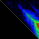
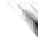
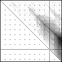
The left heatmap is shown in RGB-faux-colour decorated with a white diagonal. The center heatmap is shown in greyscale with no decorations. The right heatmap is decorated with a major diagonal, borders, lines every 100 values and ticks every ten values. Values correspond to amino acid positions where the top left is (0, 0) of the alignment.
Example Heat Maps 2: Feed Forward Back Propagation Network — Weight Training
Here’s another application of heat maps. This time we’ve visualized the training of neural network weight values. The weights are trained over 200 epochs to their final values. This visualization allows us to see the movement of weights from pseudorandom noise (top) to their final values (bottom).
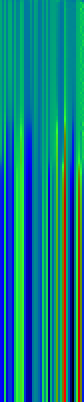


Shown above are the weight and bias values for a 2-input, 4-hidden-node, 4-hidden-node, 2-output back-propagation feed-forward ANN trained on the toy XOR-EQ problem. The maps are rendered as RGB-faux-colour (left); greyscale (center); and RGB-faux-colour decorated with horizontal lines every 25 values (=50px) (right). Without going into detail, the leftmost 12 columns bridge inputs to the first hidden layer, the next 20 columns belong to the next weight layer, and the last 10 columns bridge to the output layer.
Update: I changed the height of the images of this example to half their original height — the horizontal lines now occur every 25 values (=25px).
C# Functions
This code makes use of two C# features — (1) function delegates and (2) optional arguments. If you also crack open the main file attached, you’ll notice I also make use of a third feature — (3) named arguments. A function delegate is used so that we can define and select which heat function to use to transform a three-tuple of double values (real, min, max) into a three-tuple of byte values (R, G, B). Optional arguments are used because the function signature has a total of twelve arguments. Leaving some out with sensible default values makes a lot of sense. Finally, I use named arguments in the main function because they allow me to (1) specify my optional arguments in a logical order and (2) read which arguments have been assigned without looking at the function signature.
Heat Functions
For this code to work, heat functions must match this delegate signature. Arguments: val is the current value, min is the lowest value in the matrix and max is the highest value in the matrix; we use min and max for normalization of val.
public delegate byte[] ValueToPixel(double val, double min, double max);
This is the RGB-faux-colour function that breaks apart the domain of heats and assigns it some amount of blue, green and red.
public static byte[] FauxColourRGB(double val, double min, double max) {
    byte r = 0;
    byte g = 0;
    byte b = 0;
    val = (val - min) / (max - min);
           if(               val <= 0.2) {
        b = (byte)((val / 0.2) * 255);
    } else if(val >  0.2 &&  val <= 0.7) {
        b = (byte)((1.0 - ((val - 0.2) / 0.5)) * 255);
    }
           if(val >= 0.2 &&  val <= 0.6) {
        g = (byte)(((val - 0.2) / 0.4) * 255);
    } else if(val >  0.6 &&  val <= 0.9) {
        g = (byte)((1.0 - ((val - 0.6) / 0.3)) * 255);
    }
           if(val >= 0.5               ) {
        r = (byte)(((val - 0.5) / 0.5) * 255);
    }
    return new byte[]{r, g, b};
}
This is a far simpler greyscale function.
public static byte[] Greyscale(double val, double min, double max) {
    byte y = 0;
    val = (val - min) / (max - min);
    y = (byte)((1.0 - val) * 255);
    return new byte[]{y, y, y};
}
Heatmap Writer
The function below is split into a few logical parts: (1) we get the minimum and maximum heat values to normalize intensities against; (2) we set the pixels to the colours we want; (3) we add the decorations (borders, ticks etc.); (4) we save the file.
public static void SaveHeatmap(
    string fileName, double[,] matrix, ValueToPixel vtp,
    int pixw = 1, int pixh = 1,
    Color? decorationColour = null,
    bool drawBorder = false, bool drawDiag = false,
    int hLines = 0, int vLines = 0, int hTicks = 0, int vTicks = 0)
{
    var rows = matrix.GetLength(0);
    var cols = matrix.GetLength(1);
    var bitmap = new Bitmap(rows * pixw, cols * pixh);

    //Get min and max values ...
    var min = Double.PositiveInfinity;
    var max = Double.NegativeInfinity;
    for(int i = 0; i < matrix.GetLength(0); i ++) {
        for(int j = 0; j < matrix.GetLength(1); j ++) {
            max = matrix[i,j] > max? matrix[i,j]: max;
            min = matrix[i,j] < min? matrix[i,j]: min;
        }
    }
    //Set pixels ...
    for(int j = 0; j < bitmap.Height; j ++) {
        for(int i = 0; i < bitmap.Width; i ++) {
            var triplet = vtp(matrix[i / pixw, j / pixh], min, max);
            var color = Color.FromArgb(triplet[0], triplet[1], triplet[2]);
            bitmap.SetPixel(i, j, color);
        }
    }
    //Decorations ...
    var dc = decorationColour ?? Color.Black;
    for(int i = 0; i < bitmap.Height; i ++) {
        for(int j = 0; j < bitmap.Width; j ++) {
            if(drawBorder) {
                if(i == 0 || i == bitmap.Height -1) {
                    // Top and Bottom Borders ...
                    bitmap.SetPixel(j, i, dc);
                } else if(j == 0 || j == bitmap.Width -1) {
                    // Left and Right Borders ...
                    bitmap.SetPixel(j, i, dc);
                }
            }
            if(bitmap.Width == bitmap.Height && drawDiag && (i % 2 == 0)) {
                // Major Diagonal ... (only draw if square image +explicit)
                bitmap.SetPixel(i, i, dc);
            }
            //Zeroed lines and zeroed ticks are turned off.
            if(hLines != 0 && i % (hLines*pixh) == 0) {
                if(j % (2*pixw) == 0) {
                    //Horizontal Bars ...
                    bitmap.SetPixel(j, i, dc);
                }
            } else if(hTicks != 0 && i % (hTicks*pixh) == 0) {
                // Dots: H-Spacing
                if(vTicks != 0 && j % (vTicks*pixw) == 0) {
                    // Dots: V-Spacing
                    bitmap.SetPixel(j, i, dc);
                }
            } else if(i % (2*pixh) == 0) {
                if(vLines != 0 && j % (vLines*pixw) == 0) {
                    //Vertical Bars
                    bitmap.SetPixel(j, i, dc);
                }
            }
        }
    }

    //Save file...
    bitmap.Save(fileName, ImageFormat.Png);
    bitmap.Dispose();
}
Happy mapping 😀
Compatibility Notes: The C# code discussed was developed with Mono using Monodevelop. All code is compatible with the C#.NET 4.0 specification and is forward compatible. I’ve linked in two assemblies — (1) -r:System.Core for general C#.Net 3.5~4.0 features, and (2) r:System.Drawing to write out PNG files. If you need an overview of how to set up Monodevelop to use the System.Drawing assembly, see C Sharp PNG Bitmap Writing with System.Drawing in my notebook.
Simple Interactive Phylogenetic Tree Sketches JS+SVG+XHTML
>>> Attached: ( parse_newick_xhtml.js | draw_phylogeny.js — implementation in JS | index.html — demo with IL-1 ) <<<
>>> Attached: ( auto_phylo_diagram.tgz — includes all above, a python script, a demo makefile and IL-1 data ) <<<
In this post, I discuss a Python script I wrote that will convert a Newick Traversal and a FASTA file into a browser-viewable interactive diagram using SVG+JS+XHTML. This method is compatible with WebKit (Safari, Chrome) and Mozilla (Firefox) renderers but not Opera. XHTML doesn’t work with IE, so we’ll have to wait for massive adoption of HTML5 before I can make this work for everyone — don’t worry, it’s coming.
 To the left is what the rendered tree looks like (shown as a screen captured PNG).
I recommend looking at the demo index.xhtml above if your browser supports it now. The demo will do a far better job than text in explaining exactly what features are possible using this method.
Try clicking on the different nodes and hyperlinks in the demo — notice that the displayed alignment strips away sites (columns) that are 100% gaps so that each node displays only a profile relevant for itself.
I originally intended to explain all the details of the JavaScripts that render and drive the diagram, but I think it’d be more useful to first focus on the Python script and the data input and output from the script.
The Attached Python Script to_xhtml.py found in auto_phylo_diagram.tgz
I’ll explain how to invoke to_xhtml.py with an example below.
python to_xhtml.py IL1fasta.txt IL1tree2.txt "IL-1 group from NCBI CDD (15)" > index.xhtml
Arguments …
- Plain Text FASTA file — IL1fasta.txt
- Plain Text Newick Traversal file — IL1tree2.txt
- Title of the generated XHTML — “IL-1 group from NCBI CDD (15)”
The data I used was generated with MUSCLE with default parameters. I specified the output FASTA with -out and the output second iteration tree with -tree2.
The Attached makefile found in auto_phylo_diagram.tgz
The makefile has two actual rules. If index.html does not exist, it will be regenerated with the above Python script and IL1fasta.txt and IL1tree2.txt. If either IL1fasta.txt or IL1tree2.txt or both do not exist, these files are regenerated using MUSCLE with default parameters on the included example data file ncbi.IL1.cl00094.15.fasta.txt. Running make on the included package shouldn’t do anything since all of the files are included.
The Example Data
The example data comes from the Interleukin-1 group (cd00100) from the NCBI Conserved Domains Database (CDD).
Finally, I’ll discuss briefly the nitty gritty of the JavaScripts found as stand-alones above that are also included in the package.
Part Two of Two
As is the nature of programatically drawing things, this particular task comes with its share of prerequisites.
In a previous — Part 1, I covered Interactive Diagrams Using Inline JS+SVG+XHTML — see that post for compatibility notes and the general method (remember, this technique is a holdover that will eventually be replaced with HTML5 and that the scripts in this post are not compatible with Opera anymore).
In this current post — Part 2, I’ll also assume you’ve seen Parsing a Newick Tree with recursive descent (you don’t need to know it inside and out, since we’ll only use these functions) — if you look at the example index.html attached, you’ll see that we actually parse the Newick Traversal using two functions in parse_newick_xhtml.js — tree_builder() then traverse_tree(). The former converts the traversal to an in-memory binary tree while the latter accepts the root node of said tree and produces an array. This array is read in draw_phylogeny.js by fdraw_tree_svg() which does the actual rendering along with attaching all of the dynamic behaviour.
Parameters ( What are we drawing? )
To keep things simple, let’s focus on three requirements: (1) the tree will me sketched top-down with the root on top and its leaves below; (2) the diagram must make good use of the window width and avoid making horizontal scroll bars (unless it’s absolutely necessary); (3) the drawing function must make the diagram compatible with the overall document object model (DOM) so that we can highlight nodes and know what nodes were clicked to show the appropriate data.
Because of the second condition, all nodes in a given depth of the tree will be drawn at the same time. A horizontal repulsion will be applied so that each level will appear to be centre-justified.
General Strategy
Because we are centre-justifying the tree, we will be drawing each level of the tree simultaneously to calculate the offsets we want for each node. We perform this iteratively for each level of depth of the tree in the function fdraw_tree_svg(). Everything that is written dynamically by JavaScript goes to a div with a unique id. All of the SVG goes to id=”tree_display” and all of the textual output including raster images, text and alignments goes to id=”thoughts”. To attach behaviour to hyperlinks, whether it’s within the SVG or using standard anchor tags, the “onclick” property is defined. In this case, we always call the same function “onclick=javascript:select_node()“. This function accepts a single parameter: the integer serial number that has been clicked.
Additional Behaviour — Images and Links to Databases
After I wrote the first drafts of the JavaScripts, I decided to add two more behaviours in the current version. First, if a particular node name has the letters “GI” in it, the script will attempt to hyperlink it with the proceeding serial number against NCBI. Second, if a particular node name has the letters “PDB” in it, the script will attempt to hyperlink the following identifier against RSCB Protein Database and also pull the first thumbnail with an img tag for the 3D protein structure.
Enjoy!
This was done because I wanted to show a custom alignment algorithm to my advisors. In this demo, I’ve stripped away the custom alignment leaving behind a more general yet pleasing visualizer. I hope that the Python script and JavaScripts are useful to you. Enjoy!