On random initial weights (neural networks)
I found an old project in my archives the other day. The long and the short of it is — on occasion — if we use a three-layer back-propagation artificial neural network, initializing the hidden weight layers to larger values works better than initializing them to small values. The general wisdom is that one initializes weight layers to small values just so the bias of the system is broken, and weight values can move along, away and apart to different destination values. The general wisdom is backed by the thought that larger values can cause nets to become trapped in incorrect solutions sooner — but on this occasion, it manages to allow nets to converge more frequently.

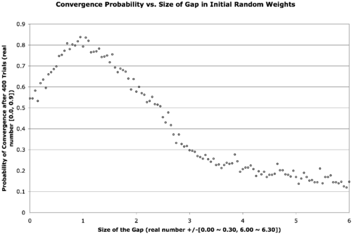
The text is a bit small, but the below explains what’s going on.
There are two neural network weight layers (2D real-valued matrices) — the first going from input-to-hidden-layer and the second going from hidden-to-output-layer. We would normally initialize these with small random values, say in the range [-0.3, 0.3]. What we’re doing here is introducing a gap in the middle of that range that expands out and forces the weights to be a bit larger. The x-axis describes the size of this gap, increasing from zero to six. The data point in the far left of the graph corresponds to a usual initialization, when the gap is zero. The gap is increased in increments of 0.05 in both the positive and negative directions for each point on the graph as we move from left to right. The next point hence corresponds to an initialization of weights in the range [-0.35, -0.05] ∨ [0.05, 0.35]. In the far right of the graph, the weights are finally randomized in the range [-6.30, -6.00] ∨ [6.00, 6.30]. The y-axis is the probability of convergence given a particular gap size. Four-hundred trials are conducted for each gap size.
The result is that the best probability of convergence was achieved when the gap size is 1.0, corresponding to weights in the random range [-1.3 -1.0] ∨ [1.0, 1.3].
What were the particular circumstances that made this work? I think this is largely dependent on the function to fit.
The Boolean function I chose was a bit of an oddball — take a look at its truth table …
| Input 1 | Input 2 | Input 3 | Output |
| 0 | 0 | 0 | 0 |
| 0 | 0 | 1 | 0 |
| 0 | 1 | 0 | 1 |
| 0 | 1 | 1 | 1 |
| 1 | 0 | 0 | 1 |
| 1 | 0 | 1 | 1 |
| 1 | 1 | 0 | 0 |
| 1 | 1 | 1 | 1 |
This comes from the function { λ : Bit_1, Bit_2, Bit_3 → (Bit_1 ∨ Bit_2) if (Bit_3) else (Bit_1 ⊕ Bit_2) }.
This function is unbalanced in the sense that it answers true more often than it answers false given the possible combinations of its inputs. This shouldn’t be too big of a problem though — we really only need any linearly inseparable function.
This project was originally done for coursework during my master’s degree. The best size for your initial weights is highly function dependent — I later found that this is less helpful (or even harmful) to problems with a continuous domain or range. It seems to work well for binary and Boolean functions and also for architectures that require recursion (I often used a gap of at least 0.6 during my master’s thesis work with the Neural Grammar Network).
Remaining parameters: training constant = 0.4; momentum = 0.4; hidden nodes = 2; convergence RMSE = 0.05 (in retrospect, using a raw count up to complete concordance would have been nicer); maximum allowed epochs = 1E5; transfer function = logistic curve.
Searching for a Continuous Bit Parity function
Update: The function being sought is better described as “continuous bit-parity” rather than “Fuzzy XOR”, the title of the post has been changed from “Fuzzy Exclusive OR (XOR)” to reflect that.
About two weeks ago, I was working on a project wherein I needed to define a continuous XOR function. The only stipulations are that (1) the function must either be binary and commutative, or it must be variadic; and (2) the function must be continuous.
In my first attempt, I used the classic arrangement of four binary NAND gates to make an XOR where each NAND gate was replaced with the expression { λ: p, q → 1.0 – pq }. The algebraic product T-norm { λ: p, q → pq } is used instead of the standard fuzzy T-norm { λ: p, q → min(p, q) } in order to keep it continuous. Unfortunately, this attempt does not preserve commutativity, so the search continued.
At this point, Dr. Kremer suggested I consider a shifted sine curve. I eventually chose the equation
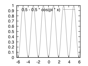
{ λ: p[1..n] → 0.5 – 0.5cos(π Σi=1npi) }.
This is shown graphically in the below figure …

# gnuplot source ...
set xrange[-2*pi:2*pi]
set output "a.eps"
set terminal postscript eps size 2.0, 1.5
plot 0.5 - 0.5 * cos(pi * x)
This can be considered a variadic function because it takes the sum of all fuzzy bits pi in a given string and treats the arguments the same no matter the number of bits n.
Whenever the sum of all bits is equal to an even number, the function returns a zero — whenever the sum is an odd number, the function returns a one. This function offers a continuous (although potentially meaningless) value between integer values of the domain and can handle bitstrings of any length.
If you’re aware of a purely binary Fuzzy XOR (instead of variadic) that is a legal extension of classic XOR, continuous, and commutative — please let me know for future reference 😀
SOM Indexing Logic
Update: Added some code too.
Brief: A classmate and I started talking about how we implemented the Kohonen Self Organizing Maps (SOM)s. I used C and indexed first the rows and the columns of the SOM before the index corresponding to the weight vectors (same as the index for the input vectors); he used C++ and indexed the weight vectors first before the columns and the rows.
Either way, we could use a three-deep array like this (switching the indexers as appropriate) …
const double low = 0.0; // minimum allowed random value to initialize weights
const double high = 1.0; // maximum allowed random value to initialize weights
const int nrows = 4; // number of rows in the map
const int ncolumns = 4; // number of columns in the map
const int ninputs = 3; // number of elements in an input vector, each weight vector

double*** weight; // the weight array

weight = calloc(nrows, sizeof(double**));
for(int r = 0; r < nrows; r ++) {
    weight[r] = calloc(ncolumns, sizeof(double*));
    for(int c = 0; c < ncolumns; c ++) {
        weight[r] = calloc(ninputs, sizeof(double));
        for(int i = 0; i < ninputs; i ++) {
            weight[r][i] =
            (((double)random() / (double)INT_MAX) * (high - low)) + low;
        }
    }
}
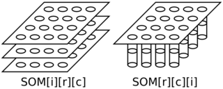
In the below diagram, the left side is a schematic of his approach and the right side is a schematic of my approach.

Figure above: SOM Indexing — Left (his): SOM indexed as input, row, column; Right (mine): SOM indexed as row, column, input.
Both schematics in the above diagram have four rows and four columns in the map where each weight (and input) vector has three elements.
I think my logic is better since we’ll often be using some distance function to evaluate how similar a weight vector is to a given input — to me, it’s natural to thus index these at the inner most nesting while looping over the rows and columns of the map.
The opposing approach was apparently used because my classmate had previously developed a matrix manipulation library. I’m actually kind of curious to take a look at it later.
SOM in Regression Data (animation)
The below animation is what happens when you train a Kohonen Self-Organizing Map (SOM) using data meant for regression instead of clustering or classification. A total of 417300 training cycles are performed — a single training cycle is the presentation of one exemplar to the SOM. The SOM has dimensions 65×65. Exemplars are chosen at random and 242 snapshots are taken in total (once every 1738 training cycles).
C & Bioinformatics: ASCII Nucleotide Comparison Circuit
Here’s a function I developed for Andre about a week ago. The C function takes two arguments. Both arguments are C characters. The first argument corresponds to a degenerate nucleotide as in the below table. The second argument corresponds to a non-degenerate nucleotide {‘A’, ‘C’, ‘G’, ‘T’} or any nucleotide ‘N’. The function returns zero if the logical intersection between the two arguments is zero. The function returns a one-hot binary encoding for the logical intersection if it exists so that {‘A’ = 1, ‘C’ = 2, ‘G’ = 4, ‘T’ = 8} and {‘N’ = 15}. All of this is done treating the lower 5-bits of the ASCII encoding for each character as wires of a circuit.
| Character | ASCII (Low 5-Bits) |
Represents | One Hot | Equals |
| A |
00001 |
A | 0001 |
1 |
| B | 00010 | CGT | 1110 |
14 |
| C | 00011 | C | 0010 |
2 |
| D | 00100 | AGT | 1101 |
13 |
| G | 00111 | G | 0100 |
4 |
| H | 01000 | ACT | 1011 |
11 |
| K |
01011 | GT | 1100 |
12 |
| M | 01101 | AC | 0011 |
3 |
| N | 01110 | ACGT | 1111 |
15 |
| R | 10010 | AG | 0101 | 5 |
| S | 10011 | GC | 0110 |
6 |
| T | 10100 | T |
1000 |
8 |
| V | 10110 | ACG |
0111 |
7 |
| W | 10111 | AT |
1001 |
9 |
| Y | 11001 | CT |
1010 |
10 |
The premise is that removing all of the logical branching and using only binary operators would make things a bit faster — I’m actually not sure if the following solution is faster because there are twelve variables local to the function scope — we can be assured that at least half of these variables will be stored outside of cache and will have to live in memory. We’d get a moderate speed boost if at all.
/*
    f():
        Bitwise comparison circuit that treats nucleotide and degenerate
        nucleotide ascii characters as mathematical sets.
        The operation performed is set i intersect j.
    arg char i:
        Primer -- accepts ascii |ABCDG HKMNR STVWY| = 15.
    arg char j:
        Sequence -- accepts ascii |ACGTN| = 5.
    return char (k = 0):
        false -- i intersect j is empty.
    return char (k > 0):
        1 -- the intersection is 'A'
        2 -- the intersection is 'C'
        4 -- the intersection is 'G'
        8 -- the intersection is 'T'
       15 -- the intersection is 'N'
    return char (undefined value):
        ? -- if any other characters are placed in i or j.
*/
char f(char i, char j) {

    // break apart Primer into bits ...
    char p = (i >> 4) &1;
    char q = (i >> 3) &1;
    char r = (i >> 2) &1;
    char s = (i >> 1) &1;
    char t =  i       &1;

    // break apart Sequence into bits ...
    char a = (j >> 4) &1;
    char b = (j >> 3) &1;
    char c = (j >> 2) &1;
    char d = (j >> 1) &1;
    char e =  j       &1;

    return

    ( // == PRIMER CIRCUIT ==
        ( // -- A --
            ((p|q|r|s  )^1) &         t |
            ((p|q|  s|t)^1) &     r     |
            ((p|  r|s|t)^1) &   q       |
            ((p|    s  )^1) &   q&r&  t |
            ((p|      t)^1) &   q&r&s   |
            ((  q|    t)^1) & p&s       |
            ((  q      )^1) & p&r&s
        )
        |
        ( // -- C --
            ((p|q|r    )^1) &       s   |
            ((p|  r|s|t)^1) &   q       |
            ((p|    s  )^1) &   q&r&  t |
            ((p|      t)^1) &   q&r&s   |
            ((  q|r    )^1) &       s&t |
            ((  q|    t)^1) & p  &r&s   |
            ((    r|s  )^1) & p&q&    t
        ) << 1
        |
        ( // -- G --
            ((  q|r|  t)^1) &       s   |
            ((p|q|  s|t)^1) &     r     |
            ((p|q      )^1) &     r&s&t |
            ((p|  r    )^1) &   q&  s&t |
            ((p|      t)^1) &   q&r&s   |
            ((  q|r    )^1) & p&    s   |
            ((  q|    t)^1) & p&    s
        ) << 2
        |
        ( // -- T --
            ((p|q|r|  t)^1) &       s   |
            ((  q|  s|t)^1) &     r     |
            ((p|  r|s|t)^1) &   q       |
            ((p|  r    )^1) &   q&  s&t |
            ((p|      t)^1) &   q&r&s   |
            ((  q      )^1) & p&  r&s&t |
            ((    r|s  )^1) & p&q&    t
        ) << 3
    )
    &
    ( // == SEQUENCE CIRCUIT ==
        ( // -- A --
            ((a|b|c|d  )^1) &         e |
            ((a|      e)^1) &   b&c&d
        )
        |
        ( // -- C --
            ((a|b|c    )^1) &       d&e |
            ((a|      e)^1) &   b&c&d
        ) << 1
        |
        ( // -- G --
            ((a|b      )^1) &     c&d&e |
            ((a|      e)^1) &   b&c&d
        ) << 2
        |
        ( // -- T --
            ((a|      e)^1) &   b&c&d   |
            ((  b|  d|e)^1) & a&  c
        ) << 3
    );
}
Andre’s eventual solution was to use a look-up table which very likely proves faster in practice. At the very least, this was a nice refresher and practical example for circuit logic using four sets of minterms (one for each one-hot output wire).
Should you need this logic to build a fast physical circuit or have some magical architecture with a dozen registers (accessible to the compiler), be my guest 😀
The Right Tool (Why I chose Java to do RSA)
Brief: I learned something valuable last week when working on this RSA encryption/decryption assignment for my Computer Security class. It’s important to be versatile when doing computer science — we must ensure we always use the most efficient tool. If we aren’t versatile, we risk taking tremendous amounts of time trying to reimplement something that already exists elsewhere.
So, what tool is the right tool to quickly throw together RSA encryption?
It turns out that Java does an excellent job. Its BigInteger class has all the ingredients you’ll ever need.
// This function generates a new probable prime ...
BigInteger p = BigInteger.probablePrime(bits, random);

// This function performs modulus inverse ...
BigInteger d = e.modInverse(phi_n);

// These functions can be used to check your work ...
BigInteger one = d.multiply(e).mod(phi_n);
BigInteger one = p.gcd(q);

// This function is at the heart of RSA ...
BigInteger C = M.modPow(d, n);
Before I looked at the Java documentation, I had plans to do this with Python and some of my classmates had plans with MATLAB. It’s not that these are inherently bad technologies — they’re just not the right tool.
As much as I have gripes with Java, I’ve got to say that this made me and a lot of my class very happy 😀
 Ed's Big Plans